Physics-Based Simulation

Polar Singular Value Decomposition

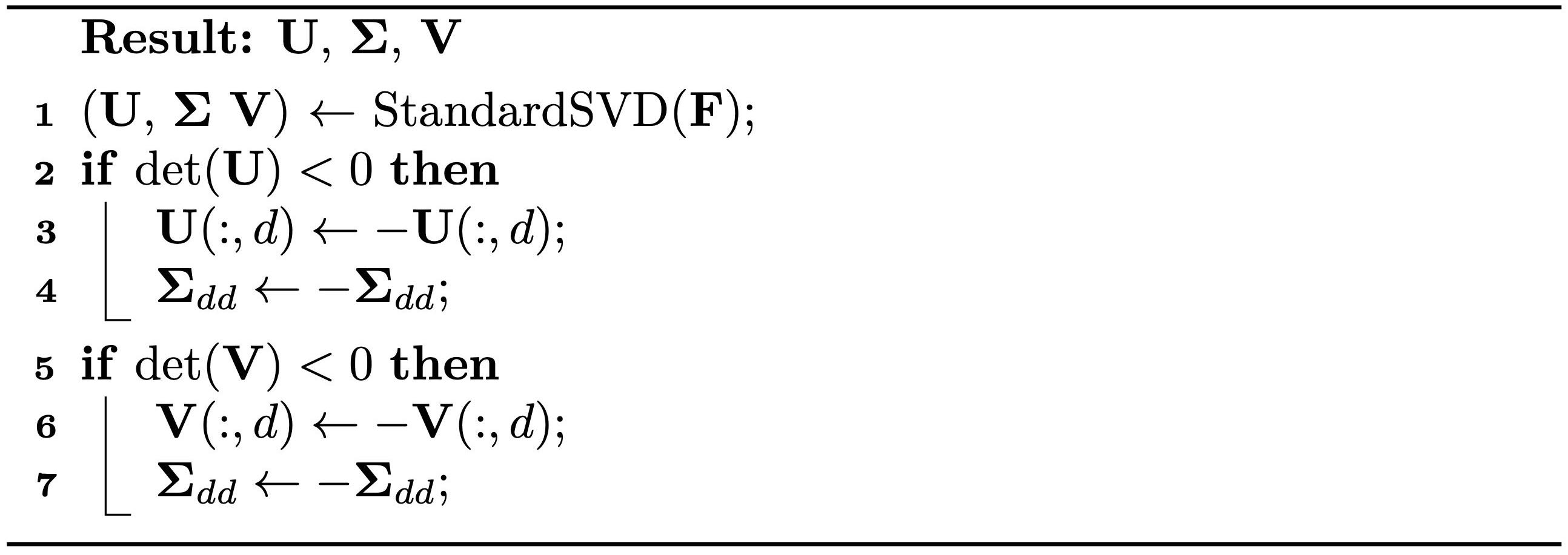
When discussing general slip boundary conditions, we introduced the usage of singular value decomposition (SVD). Here, we apply a variant known as Polar SVD (Algorithm 13.2.1) to decompose $\mathbf{F}$: $$\mathbf{F}=\mathbf{U\Sigma }{\mathbf{V}}^T,$$ where $\mathbf{U}$ and $\mathbf{V}$ are both $d\times d$ rotation matrices, and $\mathbf{\Sigma }$ is a $d\times d$ diagonal matrix. Unlike standard SVD, which ensures ${\mathbf{\Sigma }}_{ii}$ remains non-negative possibly at the expense of having $\det (\mathbf{U})=-1$ or $\det (\mathbf{V})=-1$, Polar SVD maintains $\det (\mathbf{U})=1$ and $\det (\mathbf{V})=1$, allowing ${\mathbf{\Sigma }}_{ii}$ to be negative if necessary.

Polar SVD is named for its relation to Polar decomposition, where $\mathbf{F}$ is expressed as $\mathbf{RS}$. This decomposition can be reconstructed via $\mathbf{R}=\mathbf{U}{\mathbf{V}}^T$ and $\mathbf{S}=\mathbf{V\Sigma }{\mathbf{V}}^T$, with $\mathbf{R}$ representing the closest rotation to $\mathbf{F}$ and $\mathbf{S}$ being symmetric.

The Polar SVD of $\mathbf{F}$ offers a more intuitive way to understand deformation. If we denote ${\sigma }_i={\mathbf{\Sigma }}_{ii}$, referred to as the principal stretches, we can conceptualize $\mathbf{F}$ as comprising a sequence of transformations. Initially, there is a rotation by ${\mathbf{V}}^T$, followed by scaling the dimensions by ${\sigma }_i$ along each axis, and concluding with another rotation by $\mathbf{U}$. This decomposition is applicable for all possible $\mathbf{F}$.

Polar SVD also allows for the more convenient expression of isotropic strain energy density functions using ${\sigma }_i$ exclusively. For instance, our intuitive formulation in Equation (13.1.1) can be reframed as:

$$\Psi (\mathbf{F})=\hat{\Psi }(\mathbf{\Sigma })=\frac{\mu }{4}\sum _{i=1}^d({\sigma }_i^2-1{)}^2+\frac{\lambda }{2}{\left(\prod _{i=1}^d{\sigma }_i-1\right)}^2,$$

where $J={\prod }_{i=1}^d{\sigma }_i={\sigma }_1\cdot {\sigma }_2\cdot \dots \cdot {\sigma }_d$. Moreover, the Neo-Hookean strain energy density function (Equation (13.1.2)) can be rewritten as:

$${\Psi }_{\text{NH}}(\mathbf{F})={\hat{\Psi }}_{\text{NH}}(\mathbf{\Sigma })=\frac{\mu }{2}\left(\sum _{i=1}^d{\sigma }_i^2-d\right)-\mu \ln (J)+\frac{\lambda }{2}{\ln }^2(J).$$

These two models are both consistent with linear elasticity under small deformation.

Definition 13.2.1 (Consistency to Linear Elasticity). To verify the consistency to linear elasticity of a strain energy density function $\Psi (\mathbf{F})$, we just need to check whether the following relations all hold: $$\hat{\Psi }(\mathbf{I})=0,\frac{\partial \hat{\Psi }}{\partial {\sigma }_i}(\mathbf{I})=0,\text{and}\frac{{\partial }^2\hat{\Psi }}{\partial {\sigma }_i\partial {\sigma }_j}(\mathbf{I})=2\mu {\delta }_{ij}+\lambda .$$ Here $1\le i,j\le d$, and ${\delta }_{ij}=1$ if $i=j$, otherwise it is $0$.