Physics-Based Simulation

Complete PBF Simulation

Now we combine the density constraints, tensile instability correction, and advanced fluid effects we've implemented to create a complete Position-Based Fluids simulation. The main simulation loop solves density constraints iteratively, then applies fluid-specific enhancements.

def substep():
    """Complete PBF simulation integrating all components"""
    if simulation_running[None]:
        # Standard PBD pre-solve: external forces and neighbor search
        pre_solve()           
        
        # Standard PBD constraint solving loop
        for _ in range(pbf_num_iters):
            solve_density_constraints()  # Density constraints with tensile instability correction
        
        # Standard PBD post-solve: velocity updates
        post_solve()          
        
        # Fluid-specific enhancements (beyond standard PBD)
        calculate_vorticity()           
        apply_vorticity_confinement()
        apply_xsph_viscosity()

The solver follows the standard PBD pipeline but adds fluid-specific enhancements. Density constraints are solved iteratively to enforce incompressibility, then vorticity confinement and XSPH viscosity add realistic fluid behavior.

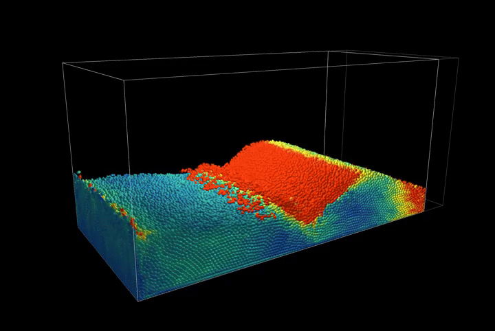
The simulation includes dynamic boundary conditions with moving walls for compression scenarios:

@ti.kernel
def move_wall():
    """Move the wall for compression scenario"""
    if wall_moving[None]:
        wall_pos[None] += wall_velocity[None] * dt
        if wall_pos[None] > wall_max_pos[None]:
            wall_pos[None] = wall_max_pos[None]
            wall_velocity[None] = -wall_velocity[None]
        elif wall_pos[None] < wall_min_pos[None]:
            wall_pos[None] = wall_min_pos[None]
            wall_velocity[None] = -wall_velocity[None]

This creates a compression scenario where the wall oscillates back and forth, showcasing the method's ability to handle complex boundary interactions.

The simulation uses spatial hashing for efficient neighbor finding:

@ti.kernel
def build_hash_grid():
    """Build spatial hash grid for neighbor finding"""
    grid_cell_counts.fill(0)
    
    for i in range(num_particles):
        cell = get_grid_cell(pos[i])
        ti.atomic_add(grid_cell_counts[cell], 1)
    
    # Build prefix sum for cell starts
    total_particles = 0
    counts_np = grid_cell_counts.to_numpy()
    starts_np = np.zeros_like(counts_np)
    for i in range(GRID_SIZE):
        for j in range(GRID_SIZE):
            for k in range(GRID_SIZE):
                starts_np[i, j, k] = total_particles
                total_particles += counts_np[i, j, k]
    grid_cell_starts.from_numpy(starts_np)

This spatial acceleration structure allows for efficient neighbor finding during density constraint solving, making the simulation scalable to large numbers of particles.

Simulation Results

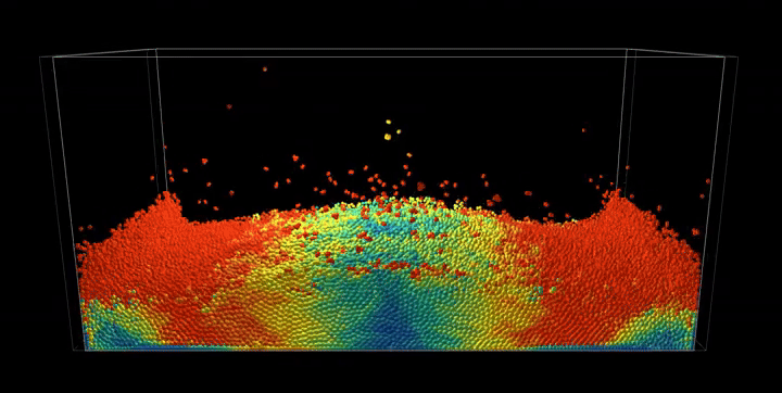
The complete PBF implementation demonstrates realistic fluid behavior through geometric constraints, showcasing incompressible flow, surface tension effects, and complex fluid interactions with dynamic boundaries.