Physics-Based Simulation

From Ground to Slope

The implementation in the Square Drop case study for horizontal grounds results in a simplified distance and distance gradient (Equation (8.3.1)) compared to that of a general half-space (Equation (7.1.1)): $$d(\mathbf{x})={\mathbf{n}}^T(\mathbf{x}-\mathbf{o}),\nabla d(\mathbf{x})=\mathbf{n},\text{and}{\nabla }^{2}d(\mathbf{x})=0.\text{\hspace{1em}(10.1.1)}$$ This is all we need for implementing the slope. Defining a normal direction and a point lying on the slope

Implementation 10.1.1 (Slope setup, simulator.py).

ground_n = np.array([0.1, 1.0])     # normal of the slope
ground_n /= np.linalg.norm(ground_n)    # normalize ground normal vector just in case
ground_o = np.array([0.0, -1.0])    # a point on the slope  

and passing them to the time integrator and barrier energy, we can modify the barrier energy value, gradient, and Hessian computation for the slope as

Implementation 10.1.2 (Slope contact barrier, BarrierEnergy.py).

import math
import numpy as np

dhat = 0.01
kappa = 1e5

def val(x, n, o, contact_area):
    sum = 0.0
    for i in range(0, len(x)):
        d = n.dot(x[i] - o)
        if d < dhat:
            s = d / dhat
            sum += contact_area[i] * dhat * kappa / 2 * (s - 1) * math.log(s)
    return sum

def grad(x, n, o, contact_area):
    g = np.array([[0.0, 0.0]] * len(x))
    for i in range(0, len(x)):
        d = n.dot(x[i] - o)
        if d < dhat:
            s = d / dhat
            g[i] = contact_area[i] * dhat * (kappa / 2 * (math.log(s) / dhat + (s - 1) / d)) * n
    return g

def hess(x, n, o, contact_area):
    IJV = [[0] * 0, [0] * 0, np.array([0.0] * 0)]
    for i in range(0, len(x)):
        d = n.dot(x[i] - o)
        if d < dhat:
            local_hess = contact_area[i] * dhat * kappa / (2 * d * d * dhat) * (d + dhat) * np.outer(n, n)
            for c in range(0, 2):
                for r in range(0, 2):
                    IJV[0].append(i * 2 + r)
                    IJV[1].append(i * 2 + c)
                    IJV[2] = np.append(IJV[2], local_hess[r, c])
    return IJV

Then for the continuous collision detection, we similarly modify the implementation to compute the large feasible initial step size for line search using $\mathbf{n}$ and $\mathbf{o}$:

Implementation 10.1.3 (Slope CCD, BarrierEnergy.py).

def init_step_size(x, n, o, p):
    alpha = 1
    for i in range(0, len(x)):
        p_n = p[i].dot(n)
        if p_n < 0:
            alpha = min(alpha, 0.9 * n.dot(x[i] - o) / -p_n)
    return alpha

Here the search direction of each node is projected onto the normal direction $\mathbf{n}$ to divide the current distance when computing the smallest step size that first brings the distance to $0$.

Finally, drawing the slope as a line from $\mathbf{o}-3\hat{n}$ to $\mathbf{o}+3\hat{n}$ where $\hat{n}=[{\mathbf{n}}_y,-{\mathbf{n}}_x]$ pointing to the inclined direction,

Implementation 10.1.4 (Slope visualization, simulator.py).

    pygame.draw.aaline(screen, (0, 0, 255), screen_projection([ground_o[0] - 3.0 * ground_n[1], ground_o[1] + 3.0 * ground_n[0]]), 
        screen_projection([ground_o[0] + 3.0 * ground_n[1], ground_o[1] - 3.0 * ground_n[0]]))   # slope

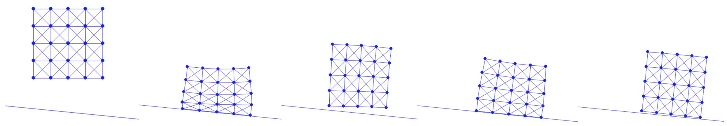
we can now simulate an elastic square dropped on a slope without friction (Figure 10.1.1).