Discrete Space

To enable numerical evaluation of the integrals in the weak form, the first step is to discretize the smooth vector fields $x$ and $Q$ . This allows them to be represented by a finite set of samples, along with appropriate interpolation functions.

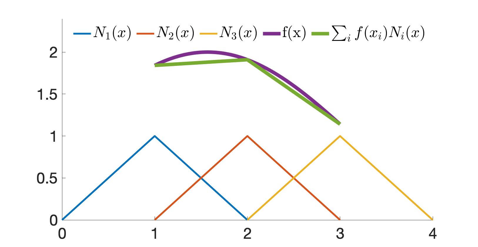
Example 17.1.1 (1D Function Interpolation). In 1D, to approximate a function $f (x)$ using three sample points $x_{1} = 1$ , $x_{2} = 2$ , $x_{3} = 3$ (Figure 17.1.1), we can use interpolation functions $N_{i} (x) = 1 - ∣ x - x_{i} ∣$ and form $f (x) \approx \sum_{i} f (x_{i}) N_{i} (x)$ .

Figure 17.1.1. With interpolation functions $N_{1} (x)$ , $N_{2} (x)$ , $N_{3} (x)$ and sample points $x_{1} = 1$ , $x_{2} = 2$ , $x_{3} = 3$ , a function $f (x)$ can be approximated as $\sum_{i} f (x_{i}) N_{i} (x)$ .

Given a set of sample points indexed by $a$ or $b$ in the simulation domain, we can approximate the test function $Q$ and the DOF $x$ as: $Q_{i} (X, t^{n}) x_{i} (X, t^{n}) \approx a \sum Q_{a ∣ i} (t^{n}) N_{a} (X) = a \sum Q_{a ∣ i}^{n} N_{a} (X), \approx b \sum x_{b ∣ i} (t^{n}) N_{b} (X) = b \sum x_{b ∣ i}^{n} N_{b} (X),$ where $Q_{a ∣ i}^{n} = Q_{a ∣ i} (t^{n})$ refers to the $i$ -th dimension of $Q$ evaluated at sample point $a$ at time $t^{n}$ , and $N_{a} (X) : Ω^{0} \to R$ is the interpolation function at sample point $a$ . In this way, we similarly have: $A_{i} (X, t^{n}) \approx b \sum A_{b ∣ i} (t^{n}) N_{b} (X) = b \sum A_{b ∣ i}^{n} N_{b} (X) . (17.1.1)$ Plugging these discretizations into the weak form (Equation (17.1)) and expressing summations with the index notation, we obtain: $\int_{Ω^{0}} R (X, 0) Q_{a ∣ i}^{n} N_{a} (X) A_{b ∣ i}^{n} N_{b} (X) d X = \int_{\partial Ω^{0}} Q_{a ∣ i}^{n} N_{a} (X) T_{i} (X, t^{n}) d s (X) - \int_{Ω^{0}} Q_{a ∣ i}^{n} N_{a, j} (X) P_{ij} (X, t^{n}) d X .$ On the left-hand side, we see that the sample values $Q_{a ∣ i}^{n}$ and $A_{b ∣ i}^{n}$ are in fact independent of $X$ , so we can move them out of the integral and obtain: $M_{ab} Q_{a ∣ i}^{n} A_{b ∣ i}^{n} = \int_{\partial Ω^{0}} Q_{a ∣ i}^{n} N_{a} (X) T_{i} (X, t^{n}) d s (X) - \int_{Ω^{0}} Q_{a ∣ i}^{n} N_{a, j} (X) P_{ij} (X, t^{n}) d X$ where $M_{ab} = \int_{Ω^{0}} R (X, 0) N_{a} (X) N_{b} (X) d X (17.1.2)$ is the mass matrix.

Remark 17.1.1 (Mass Matrix Properties). The mass matrix $M$ (Equation (17.1.2)) is symmetric and positive semi-definite because it can be expressed as: $\int_{Ω^{0}} B B^{T} d X,$ where $B_{i} = R (X, 0) N_{i} (X)$ . Thus, for any vector $z$ , $z^{T} M z = \int_{Ω^{0}} (z^{T} B)^{2} d X \geq 0.$ In practice, this mass matrix may be singular. To address this, we typically use a "mass lumping" strategy to approximate the mass matrix with a diagonal and positive definite form. This is achieved by summing each row and defining: $M_{ab}^{lump} = δ_{ab} c \sum M_{a c} .$

After spatial discretization, the solution of the weak form (Equation (17.1)) is confined to $d$ $n$ -dimensional function spaces, where $n$ represents the number of sample points, assuming all interpolation functions are mutually orthogonal. This means that there could be continuous solutions to the weak form outside of our solution space. In such cases, we can only provide an approximate solution based on the chosen sample points and interpolation functions.

Definition 17.1.1 (Orthogonal Functions). Similar to the orthogonality of two vectors $a$ and $b$ , defined as $a^{T} b = 0$ , the orthogonality of two functions $f (x)$ and $g (x)$ is defined as: $\int f (x) g (x) d x = 0.$ Just as a basis of vectors can span a finite-dimensional space, orthogonal functions can form an infinite basis for a function space. Conceptually, the integral above is analogous to a vector dot product.

That being said, to generate equations solvable for the unknowns, the arbitrary test function $Q$ does not need to cover all possibilities to produce an infinite number of equations. Instead, we only need to produce a finite set of equations that spans the entire solution space. Therefore, for $\overset{a}{^}$ traversing all sample points, and $\hat{i} = 1, 2, \dots, d$ , we can assign the test function: $Q_{a ∣ i}^{n} = {1, 0, a = \overset{a}{^} and i = \hat{i} otherwise$ to obtain $n d$ equations: $M_{\overset{a}{^} b} A_{b ∣ \hat{i}}^{n} = \int_{\partial Ω^{0}} N_{\overset{a}{^}} (X) T_{\hat{i}} (X, t^{n}) d s (X) - \int_{Ω^{0}} N_{\overset{a}{^}, j} (X) P_{\hat{i} j} (X, t^{n}) d X, (17.1.3)$ resulting in $n d$ unknowns and $n d$ equations, bringing us closer to the discrete form.

The two integrals on the right side of Equation (17.1.3) can be evaluated analytically or using quadrature rules, depending on the specific choice of interpolation functions. We will discuss these in detail in future lectures.