Physics-Based Simulation

Direct Solver

Direct solvers are a class of algorithms designed to compute the exact solution to a linear system in a finite number of steps, up to numerical precision. In the context of optimization and simulation, the coefficient matrix $A$ is often symmetric positive definite (SPD), making direct solvers both robust and efficient for moderate-sized problems.

Forward and Backward Substitution for Triangular Matrices

Solving $Ax=b$ is particularly straightforward when $A$ is triangular. If $A$ is lower triangular, i.e. $$\left[\begin{array}{cccc}{a}_{11}& 0& \cdots & 0\\ a_{21}& a_{22}& \cdots & 0\\ ⋮& ⋮& \ddots & 0\\ a_{n1}& a_{n2}& \cdots & a_{nn}\end{array}\right]\left[\begin{array}{c}{x}_1\\ x_2\\ ⋮\\ x_n\end{array}\right]=\left[\begin{array}{c}{b}_1\\ b_2\\ ⋮\\ b_n\end{array}\right].\text{\hspace{1em}(34.1.1)}$$ the system can be solved by forward substitution. The $i$-th variable is solved as: $$x_i=\frac{1}{a_{ii}}\left(b_i-\sum _{j=1}^{i-1}{a}_{ij}{x}_j\right),i=1,\dots ,n.\text{\hspace{1em}(34.1.2)}$$ This process proceeds from $i=1$ to $n$, using previously computed $x_j$ for $j<i$.

If $A$ is upper triangular, the system is solved by backward substitution: $$x_i=\frac{1}{a_{ii}}\left(b_i-\sum _{j=i+1}^n{a}_{ij}{x}_j\right),i=n,n-1,\dots ,1.\text{\hspace{1em}(34.1.3)}$$ This process proceeds from $i=n$ down to $1$, using already computed $x_j$ for $j>i$.

Cholesky Decomposition

For general SPD matrices, we can reduce the problem to triangular systems using the Cholesky decomposition. Given $A$ SPD, we can factor $A=L{L}^T$, where $L$ is lower triangular.

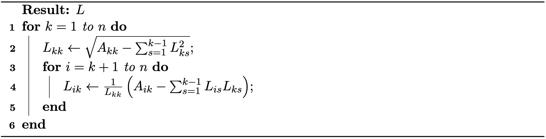
Method 34.1.1 (Cholesky Decomposition). Given a symmetric positive definite matrix $A$, the Cholesky decomposition computes a lower triangular matrix $L$ such that $A=L{L}^T$. The algorithm is as follows:

Once the decomposition is computed, solving $Ax=b$ reduces to two triangular systems:

1. Forward substitution: Solve $Ly=b$ for $y$.
2. Backward substitution: Solve $L^{T}x=y$ for $x$.

Cholesky decomposition takes advantage of the symmetry and positive definiteness of $A$, reducing both computational cost and memory usage compared to general-purpose methods like LU decomposition. Direct solvers are widely used when the system size is not too large, or when high accuracy is required for ill-conditioned systems. For very large or highly sparse systems, iterative solvers may be preferred, as discussed in the next section.