Physics-Based Simulation

Spatial and Temporal Discretizations

In representing solid geometries, we employ a mesh structure. We can further simplify the representation by connecting nodes on the mesh with edges. To facilitate this process, especially for geometries like squares, we can script a mesh generator. This generator allows for specifying both the side length of the square and the desired resolution of the mesh.

Implementation 4.1.1 (Square Mesh Generation, square_mesh.py).

import numpy as np
import os

def generate(side_length, n_seg):
    # sample nodes uniformly on a square
    x = np.array([[0.0, 0.0]] * ((n_seg + 1) ** 2))
    step = side_length / n_seg
    for i in range(0, n_seg + 1):
        for j in range(0, n_seg + 1):
            x[i * (n_seg + 1) + j] = [-side_length / 2 + i * step, -side_length / 2 + j * step]
    
    # connect the nodes with edges
    e = []
    # horizontal edges
    for i in range(0, n_seg):
        for j in range(0, n_seg + 1):
            e.append([i * (n_seg + 1) + j, (i + 1) * (n_seg + 1) + j])
    # vertical edges
    for i in range(0, n_seg + 1):
        for j in range(0, n_seg):
            e.append([i * (n_seg + 1) + j, i * (n_seg + 1) + j + 1])
    # diagonals
    for i in range(0, n_seg):
        for j in range(0, n_seg):
            e.append([i * (n_seg + 1) + j, (i + 1) * (n_seg + 1) + j + 1])
            e.append([(i + 1) * (n_seg + 1) + j, i * (n_seg + 1) + j + 1])

    return [x, e]

In the code, n_seg represents the number of edges along each side of the square. The nodes are uniformly distributed across the square and interconnected through horizontal, vertical, and diagonal edges. For instance, calling generate(1.0, 4) constructs a mesh as depicted in Figure 4.1.1. This implementation utilizes the array data structures from the Numpy library, which provides convenient methods for handling the vector algebra required in subsequent steps.

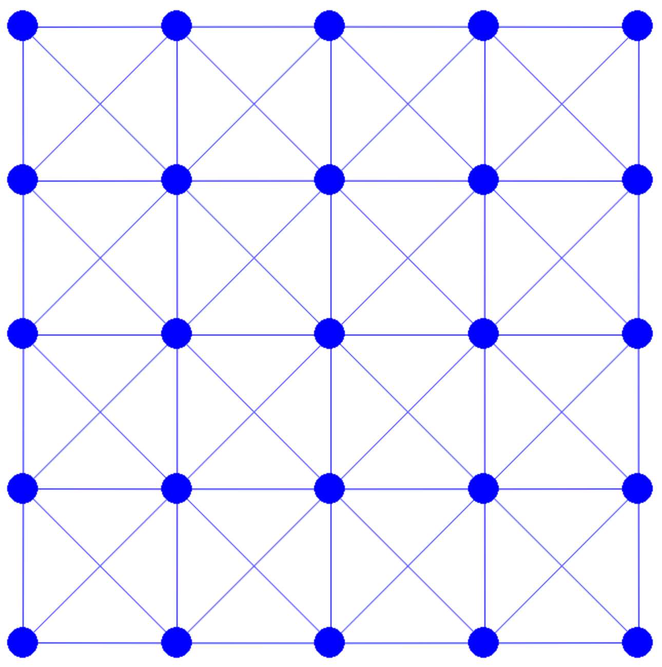
For temporal discretization, our approach is the implicit Euler method. The Incremental Potential, which needs to be minimized in time step \(n\), is represented as follows: $$E(x)=\frac{1}{2}\Vert x-(x^n+h{v}^n){\Vert }_M^2+h^{2}P(x).\text{\hspace{1em}(4.1.1)}$$ Next, our focus shifts to implementing the calculations for the energy value, gradient, and Hessian for both the inertia term and the potential energy \(P(x)\).