The Tunneling Issue
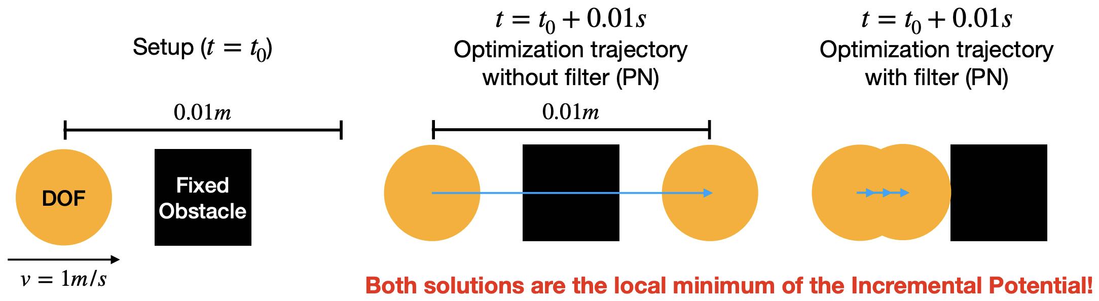
Example 8.1.1 (Tunneling). Let's consider a simple illustrative example. Without external forces like gravity, for a particle (no elasticity) at \(\mathbf{x}_0 = (0, 0)\) with mass \(m\) and initial velocity \(\mathbf{v}_0 = (1, 0)\) hitting a fixed square obstacle centered at \((0.005, 0) \), the Incremental Potential minimization problem for the first time step is Since \(\hat{d}\) is usually set small enough such as \(10^{-4}m\) in this case, the barrier potential \(P_b(\mathbf{x})\) is not yet active at \(\mathbf{x}_0\) as the particle is not touching the obstacle. This makes the problem in Equation (8.1.1) quadratic, and our projected Newton (PN) method (Algorithm 3.3.1) will produce a search direction at the first iteration, which directly leads to the global minimum of the Incremental Potential at \(\mathbf{x}_0 + h\mathbf{v}_0\) after line search. Taking \(h=0.01s\) (Figure 8.1.1), the particle will tunnel through the obstacle. However, scenarios where particles pass through obstacles due to large time steps are clearly unrealistic, as the expected physical behavior is for the particle to collide with the obstacle and either stop or bounce back.
From Example 8.1.1, we understand that simply ensuring the signed distances to be non-negative at the final solution is inadequate, especially in scenarios involving large time step sizes, high-speed impacts, or thin obstacles. These conditions can lead to inaccuracies and unrealistic outcomes in simulations.
The Incremental Potential Contact (IPC) method addresses this issue by ensuring that distances remain non-zero across the entire motion trajectory of solids. This approach is crucial for maintaining the physical accuracy and realism of the simulation.
But what exactly do we mean by "motion trajectory" in the context of discrete time integration? We will explain this next.