Physics-Based Simulation

Explicit Time Integration

Explicit time integration schemes provide a direct method to calculate \(x^{n+1},v^{n+1}\) by substituting known values into simple formulas, which is why these are called explicit. This section focuses on two basic explicit schemes: Forward Euler and Symplectic Euler methods.

Forward Euler

To convert our continuous-time system to a discrete form, we employ the forward difference approximation. In this approximation, the derivative \((\frac{\mathbf{d} x}{\mathbf{d} t})^n\) is estimated as \(\frac{x^{n+1} - x^n}{\Delta t}\), and likewise, \((\frac{\mathbf{d} v}{\mathbf{d} t})^n\) as \(\frac{v^{n+1} - v^n}{\Delta t}\). The superscript \(n\) represents the state variables at the \(n\)th timestep. Consequently, the discrete version of our system is expressed as: $$\begin{array}{rl}\frac{x^{n+1}-x^n}{\Delta t}& =v^n,\\ M\frac{v^{n+1}-v^n}{\Delta t}& =f^n.\end{array}\text{\hspace{1em}(1.4.1)}$$ Assuming a constant mass over time, these equations provide a clear mechanism to update our state variables. Knowing the current values \(x^n\), \(v^n\), and \(f^n\) at timestep \(n\), we can directly determine their values at the next timestep, \(n+1\).

Method 1.4.1 (Forward Euler Time Integration for Newton's Second Law). In the Forward Euler method, the state variables \(x^{n+1}\) and \(v^{n+1}\) at the next time step \(n+1\) are calculated based on the current values \(x^n\) and \(v^n\). The update rules are given by: $$\begin{array}{rl}{x}^{n+1}& =x^n+\Delta t{v}^n,\\ v^{n+1}& =v^n+\Delta t{M}^{-1}{f}^n.\end{array}\text{\hspace{1em}(1.4.2)}$$ Here, \(\Delta t\) represents the time step size, \(M\) is the mass matrix, and \(f^n\) is the force at the current time step \(n\).

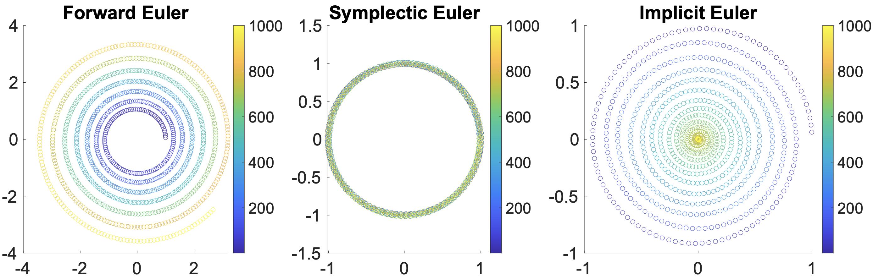
The forward Euler method is considered unconditionally unstable, implying that irrespective of the chosen small time step \(\Delta t\), the numerical solution will eventually grow significantly (explode) for equations with nonconstant \(f\), while the exact solution remains unaffected (refer to Figure 1.4.1, left).

Symplectic Euler

If we put superscript \(n+1\) on \(v\) in the position derivative discretization while keeping the velocity derivative the same, we get a new update rule:

Method 1.4.2 (Symplectic Euler Time Integration for Newton's Second Law). Given the current state variables, the mass matrix, and the time step size from \(t^n\) to \(t^{n+1}\), $$\begin{array}{rl}{x}^{n+1}& =x^n+\Delta t{v}^{n+1}\\ v^{n+1}& =v^n+\Delta t{M}^{-1}{f}^n,\end{array}\text{\hspace{1em}(1.4.3)}$$ where \(n=0,1,2,\dots\).

With a minor alteration, the integration becomes conditionally stable. This implies that if \(\Delta t\) remains within a problem-specific limit, we can effectively confine the numerical error of the solution. Moreover, the Symplectic Euler method exhibits an appealing trait of system energy preservation, as demonstrated in the middle of the figure below.