In everyday life, solid objects are perceived as continuous. Yet, in the digital world of computers, where we use discrete numbers for representation, a range of interesting methods arises.
One method is parametrization. Consider a 3D sphere, which can be described as {x∈R3∣∥x−c∥≤r,c∈R3,r>0}, centered at point \( \mathbf{c} \) with radius \( r \). This approach extends beyond spheres to include shapes like half-spaces, boxes, ellipsoids, tori, and others, characterized by their interior using functions such as signed distances. However, parametrization faces challenges when handling complex geometries that are frequently encountered in real-world scenarios. An emerging exception to this limitation is the use of advanced neural representations employing neural networks. These newer methods show promise in effectively representing more intricate geometrical forms.
An alternative is representing with sampling. This involves choosing points on and inside the object. But points alone aren't enough; we typically need to establish connectivity between them to define the object’s boundaries for applications like rendering and 3D printing. Monitoring how a cluster of points shifts over time also helps in measuring deformation.
In continuum mechanics, an object is seen as having a continuous density field. Digitally, this continuity must be represented discretely, usually through defining the connectivity of the solid's geometry.
Remark 1.1.1 (Other Solid Representations).
There are other methods for representing solid geometries, such as voxel-based approaches. These methods divide the space into a 3D grid of small boxes, or voxels, with each voxel representing a segment of the object, similar to pixels in a 2D image. Voxel-based methods are advantageous for several reasons. Firstly, they can act as a discrete level set representation, capable of modeling complex geometries and tracking their evolution over time. Each voxel contains information about its position relative to the object's surface, offering an efficient discrete approximation of the continuous level set function. This is beneficial for algorithms involved in surface evolution, shape optimization, and collision detection. Secondly, voxel-based approaches are conducive to Constructive Solid Geometry (CSG) operations. This technique in solid modeling uses Boolean operators to combine simpler shapes into complex 3D models. The voxelized framework allows for straightforward and efficient execution of operations like union, intersection, and difference on the voxel grid. This enables the easy creation and modification of intricate shapes.
Example 1.1.1 (Mesh).
The method of creating a mesh by directly connecting points with edges or triangles is a popular technique in computational geometry. This concept is illustrated in the accompanying figure, where the left and middle images show two different meshes. Notably, even though these meshes utilize the same sampled points or nodes, they have distinct connectivities, resulting in different shapes. The rightmost mesh in the figure demonstrates a transformation from one shape to another. This mesh represents a deformation of the middle mesh, achieved by vertically compressing its upper half.
Figure 1.1.1. Mesh
Example 1.1.2 (Particle and Grid).
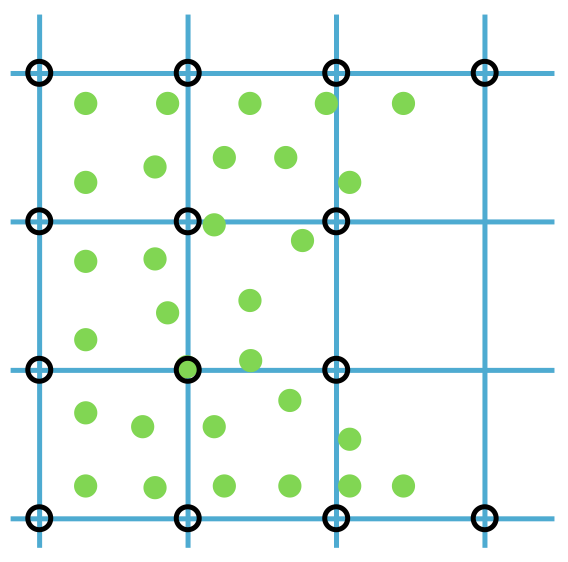
By implementing a uniform grid structure in our spatial representation, we record the extent of solid matter at each node location. This allows us to use our sampled points to calculate the density of the solid at each grid node. This method is beneficial for quantifying the solid's distribution within the grid and for establishing a network of connectivity among the original sampled points. Refer to the accompanying figure for a visual demonstration of this concept. In the figure, the sampled points are depicted as green dots. The grid nodes, where we record solid densities, are shown as black circles. These nodes are connected through the grid, illustrated with blue lines.
Figure 1.1.2. Particle and grid
In the field of modern solid simulation, the described methods of defining connectivity are crucial. The first method, establishing connections through a mesh of edges or triangles, is foundational to Finite Element Method (FEM) simulators. The second approach, which involves using a uniform grid to compute solid density and establish connectivity, is integral to Material Point Method (MPM) simulators [Jiang et al. 2016]. This book largely concentrates on the former method, delving into the intricacies of FEM. The mesh-based structure of FEM is particularly effective in handling complex domains by breaking them down into simpler elements. This makes FEM an essential tool in the study and simulation of deformable solids, and understanding its nuances is vital for those engaged in this area of study.
At first glance, the use of two representations of solid geometry in the MPM might appear redundant. Yet, this dual approach gives MPM a significant edge, especially in simulating dynamic events like solid fractures. In such cases, FEM would necessitate meticulous modification of the edges and elements that define the original connectivity to accurately depict the damage. In contrast, MPM efficiently handles these scenarios. The uniform grid naturally accommodates the separation of body parts in a fracture, as the lack of material at fracture nodes leads to an automatic disconnection of adjacent grid nodes. This attribute allows MPM to excel in managing changes in solid topology.
However, when it comes to simulation accuracy control, the Finite Element Method (FEM) excels. FEM operates directly on the mesh, obviating the need for constant information transfer, thus ensuring greater precision. This level of accuracy makes FEM an invaluable resource in the precise simulation of deformable solids, which is the primary emphasis of this book.
The technique of consolidating coordinates of each sampled point into an extended vector, denoted as \( x\in\mathbb{R}^{dn} \) (refer to the figure below), provides an effective means to describe a specific geometric configuration, given a constant connectivity. In this representation, \(d\) indicates the dimension of space (1, 2, or 3), and \(n\) represents the total number of points. Similarly, attributes like velocity, acceleration, and forces at each sample point can be amalgamated into corresponding extended vectors, symbolized as \(v\), \(a\), and \(f\) respectively. This organized approach to data presentation not only aids in comprehensively understanding the various parameters and their interrelations but also streamlines the mathematical formulation of the simulation process.