Physics-Based Simulation

Slope Friction

Now to implement friction for the slope, we start by implementing the functions that calculate $f_0(\Vert {\bar{v}}_k\Vert \hat{h})$, $f_1(\Vert {\bar{v}}_k\Vert )/\Vert {\bar{v}}_k\Vert$, and $(f_1^{\prime }(\Vert {\bar{\mathbf{v}}}_k\Vert )\Vert {\bar{\mathbf{v}}}_k\Vert -f_1(\Vert {\bar{\mathbf{v}}}_k\Vert ))/\Vert {\bar{\mathbf{v}}}_k{\Vert }^2$ according to Equation (9.2.2), Equation (9.2.5), and Equation (9.2.6) respectively.

Implementation 10.2.1 (Friction helper functions, FrictionEnergy.py).

import numpy as np
import utils

epsv = 1e-3

def f0(vbarnorm, epsv, hhat):
    if vbarnorm >= epsv:
        return vbarnorm * hhat
    else:
        vbarnormhhat = vbarnorm * hhat
        epsvhhat = epsv * hhat
        return vbarnormhhat * vbarnormhhat * (-vbarnormhhat / 3.0 + epsvhhat) / (epsvhhat * epsvhhat) + epsvhhat / 3.0

def f1_div_vbarnorm(vbarnorm, epsv):
    if vbarnorm >= epsv:
        return 1.0 / vbarnorm
    else:
        return (-vbarnorm + 2.0 * epsv) / (epsv * epsv)

def f_hess_term(vbarnorm, epsv):
    if vbarnorm >= epsv:
        return -1.0 / (vbarnorm * vbarnorm)
    else:
        return -1.0 / (epsv * epsv)

With these terms available, we can then implement the semi-implicit friction energy value, gradient, and Hessian computations according to Equation (9.2.1), Equation (9.2.3), and Equation (9.2.4) respectively.

Implementation 10.2.2 (Friction value, gradient, and Hessian, FrictionEnergy.py).

def val(v, mu_lambda, hhat, n):
    sum = 0.0
    T = np.identity(2) - np.outer(n, n) # tangent of slope is constant
    for i in range(0, len(v)):
        if mu_lambda[i] > 0:
            vbar = np.transpose(T).dot(v[i])
            sum += mu_lambda[i] * f0(np.linalg.norm(vbar), epsv, hhat)
    return sum

def grad(v, mu_lambda, hhat, n):
    g = np.array([[0.0, 0.0]] * len(v))
    T = np.identity(2) - np.outer(n, n) # tangent of slope is constant
    for i in range(0, len(v)):
        if mu_lambda[i] > 0:
            vbar = np.transpose(T).dot(v[i])
            g[i] = mu_lambda[i] * f1_div_vbarnorm(np.linalg.norm(vbar), epsv) * T.dot(vbar)
    return g

def hess(v, mu_lambda, hhat, n):
    IJV = [[0] * 0, [0] * 0, np.array([0.0] * 0)]
    T = np.identity(2) - np.outer(n, n) # tangent of slope is constant
    for i in range(0, len(v)):
        if mu_lambda[i] > 0:
            vbar = np.transpose(T).dot(v[i])
            vbarnorm = np.linalg.norm(vbar)
            inner_term = f1_div_vbarnorm(vbarnorm, epsv) * np.identity(2)
            if vbarnorm != 0:
                inner_term += f_hess_term(vbarnorm, epsv) / vbarnorm * np.outer(vbar, vbar)
            local_hess = mu_lambda[i] * T.dot(utils.make_PSD(inner_term)).dot(np.transpose(T)) / hhat
            for c in range(0, 2):
                for r in range(0, 2):
                    IJV[0].append(i * 2 + r)
                    IJV[1].append(i * 2 + c)
                    IJV[2] = np.append(IJV[2], local_hess[r, c])
    return IJV

Note that in Numpy, matrix-matrix and matrix-vector products are realized by the dot() function. For implicit Euler, $v=(x-x^n)/h$ and so $\hat{h}=h$. Here mu_lambda stores $\mu {\lambda }_k^n$ for each node, where the normal force magnitude ${\lambda }_k^n$ is calculated using $x^n$ at the beginning of each time step.

Implementation 10.2.3 (Use mu and lambda, time_integrator.py).

def step_forward(x, e, v, m, l2, k, n, o, contact_area, mu, is_DBC, h, tol):
    x_tilde = x + v * h     # implicit Euler predictive position
    x_n = copy.deepcopy(x)
    mu_lambda = BarrierEnergy.compute_mu_lambda(x, n, o, contact_area, mu)  # compute mu * lambda for each node using x^n

    # Newton loop

Implementation 10.2.4 (Compute mu and lambda, BarrierEnergy.py).

def compute_mu_lambda(x, n, o, contact_area, mu):
    mu_lambda = np.array([0.0] * len(x))
    for i in range(0, len(x)):
        d = n.dot(x[i] - o)
        if d < dhat:
            s = d / dhat
            mu_lambda[i] = mu * -contact_area[i] * dhat * (kappa / 2 * (math.log(s) / dhat + (s - 1) / d))
    return mu_lambda

Since the slope is static, and the normal direction is the same everywhere, $T$ is constant and so can be discretized accurately.

Finally, we set friction coefficient $\mu$ and pass it to the time integrator where we add friction energy to model semi-implicit friction on the slope.

mu = 0.11        # friction coefficient of the slope

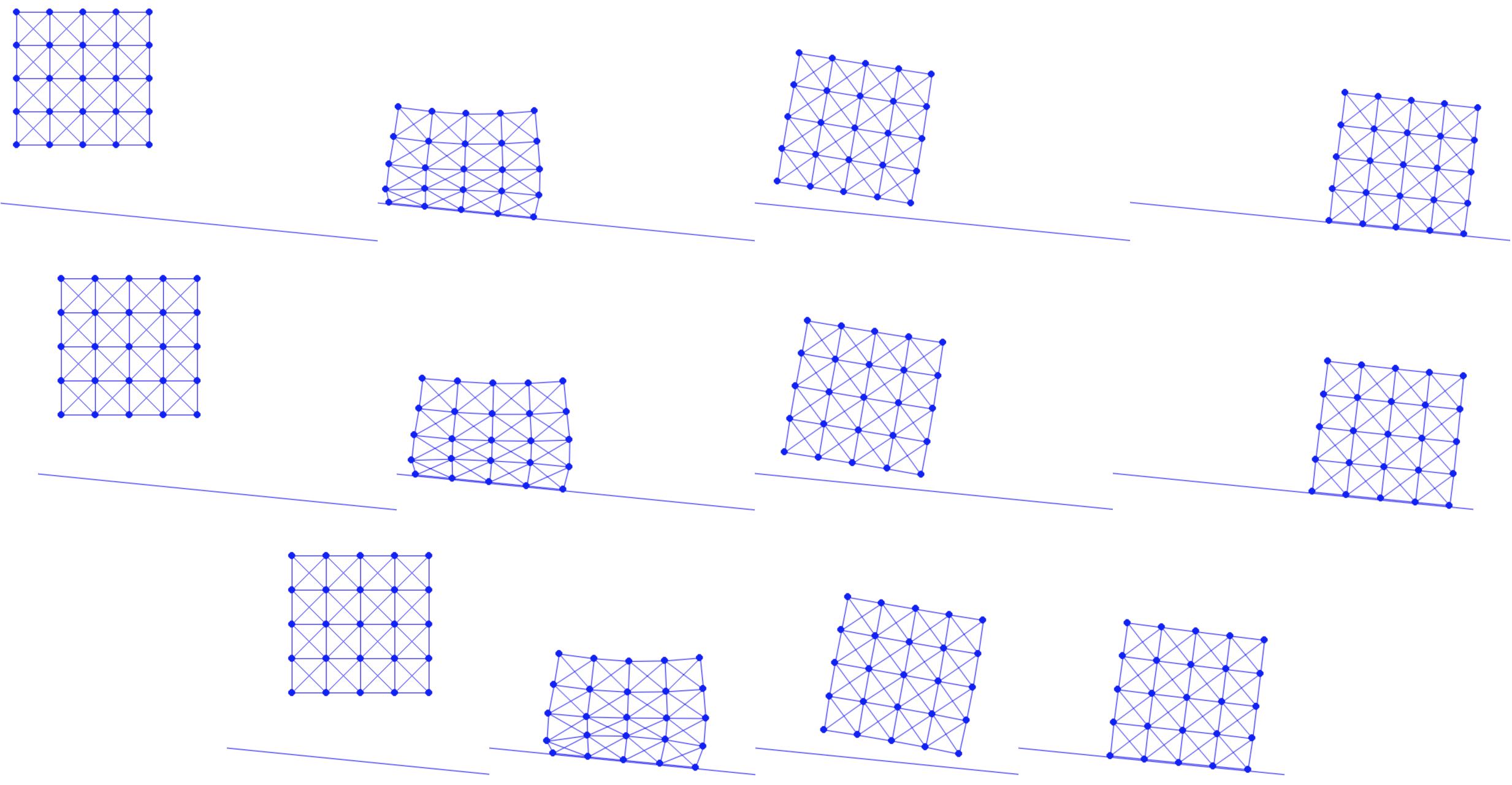
Now we are ready to test the simulation with different friction coefficients. Since our slope has an inclined angle $\theta$ with $\tan (\theta )=0.1$, we test $\mu =0.1$, $0.11$, and $0.2$ (Figure 10.2.1). Here we see that when $\mu =0.1$, the critical value that provides dynamic friction forces in the same magnitude with that of the gravity component on the slope, the square keeps sliding after gaining the initial momentum (Figure 10.2.1 top). When we set $\mu =0.11$, right above the critical value, the square slides a while and then stopped, showing that static friction is properly resolved (Figure 10.2.1 middle). With $\mu =0.2$, the square stops even earlier (Figure 10.2.1 bottom).