Physics-Based Simulation

Signed Distances

The Incremental Potential Contact (IPC) method is designed to ensure non-interpenetration in solids of any codimension by maintaining the unsigned distances between solid boundaries above zero throughout their movement. This approach is robust as it applies universally, irrespective of the solid's specific characteristics.

However, when signed distances are accessible, the application of IPC becomes not only straightforward but also more streamlined. Signed distances extend the concept of unsigned distances to encompass solid geometries with closed boundaries. With IPC enforcing non-interpenetration, the possibility of negative distances inside a solid is eliminated. Therefore, in scenarios where signed distances remain non-negative (including the state of being exactly zero), it's an indication of successful non-interpenetration.

Definition 7.1.1 (Codimension). If \(W\) is a linear subspace of a finite-dimensional vector space \(V\), then the codimension of \(W\) in \(V\) is the difference between their dimensions: $$\text{codim}(W)=\text{dim}(V)-\text{dim}(W).$$ For example, in 3D, a surface has codimension \(1\), and a line has codimension \(2\). In computer graphics, when simulating cloth and hair, codimension 1 and 2 geometry representations are often applied respectively for efficiency. However, their signed distances are not well-defined. This also explains why unsigned distances are more general for modeling solid contact.

In a previous section, we explored various methods for representing solid geometries. One notable approach is the analytical representation. For instance, a 3D ball centered at \( \mathbf{c} \) with radius \( r \) can be analytically described by the parameterization:

$$\{\mathbf{x}\in {\mathbb{R}}^3|\Vert \mathbf{x}-\mathbf{c}\Vert \le r,\mathbf{c}\in {\mathbb{R}}^3,r>0\}.$$

This principle of defining solid geometries extends beyond simple spheres. Many other shapes, such as half-spaces, boxes, ellipsoids, and tori, can be similarly parameterized. The key to these parameterizations lies in defining the "interior" of these objects, which can often be achieved through functions like signed distances. These functions provide a versatile tool for describing a wide range of simple and complex shapes in a concise and mathematical manner.

Example 7.1.1 (Ball Signed Distance Function). The signed distance function \(d(\mathbf{x})\) and its derivatives of a ball centered at \(\mathbf{c}\) with radius \(r\) can be defined as $$\begin{array}{rl}& d(\mathbf{x})=\Vert \mathbf{x}-\mathbf{c}\Vert -r,\nabla d(\mathbf{x})=\frac{\mathbf{x}-\mathbf{c}}{\Vert \mathbf{x}-\mathbf{c}\Vert },\\ & \text{and}{\nabla }^{2}d(\mathbf{x})=\frac{\Vert \mathbf{x}-\mathbf{c}{\Vert }^{2}I-(\mathbf{x}-\mathbf{c})(\mathbf{x}-\mathbf{c}{)}^T}{\Vert \mathbf{x}-\mathbf{c}{\Vert }^3}.\end{array}$$

Example 7.1.2 (Half-Space Signed Distance Function). The signed distance function \(d(\mathbf{x})\) and its derivatives of a half-space with normal \(\mathbf{n}\) and \(d(\mathbf{o}) = 0\) can be defined as $$d(\mathbf{x})={\mathbf{n}}^T(\mathbf{x}-\mathbf{o}),\nabla d(\mathbf{x})=\mathbf{n},\text{and}{\nabla }^{2}d(\mathbf{x})=0.\text{\hspace{1em}(7.1.1)}$$

Representing more intricate geometries, like those commonly encountered in real-life scenarios, can be a challenging task due to their complexity. An effective alternative to intricate parameterizations is the use of a uniform Euclidean grid. This grid serves as a storage mechanism for the signed distances of a solid object, with these distances precomputed at each grid node. When the distance at any arbitrary point within the solid is required, interpolation can be applied to the grid data.

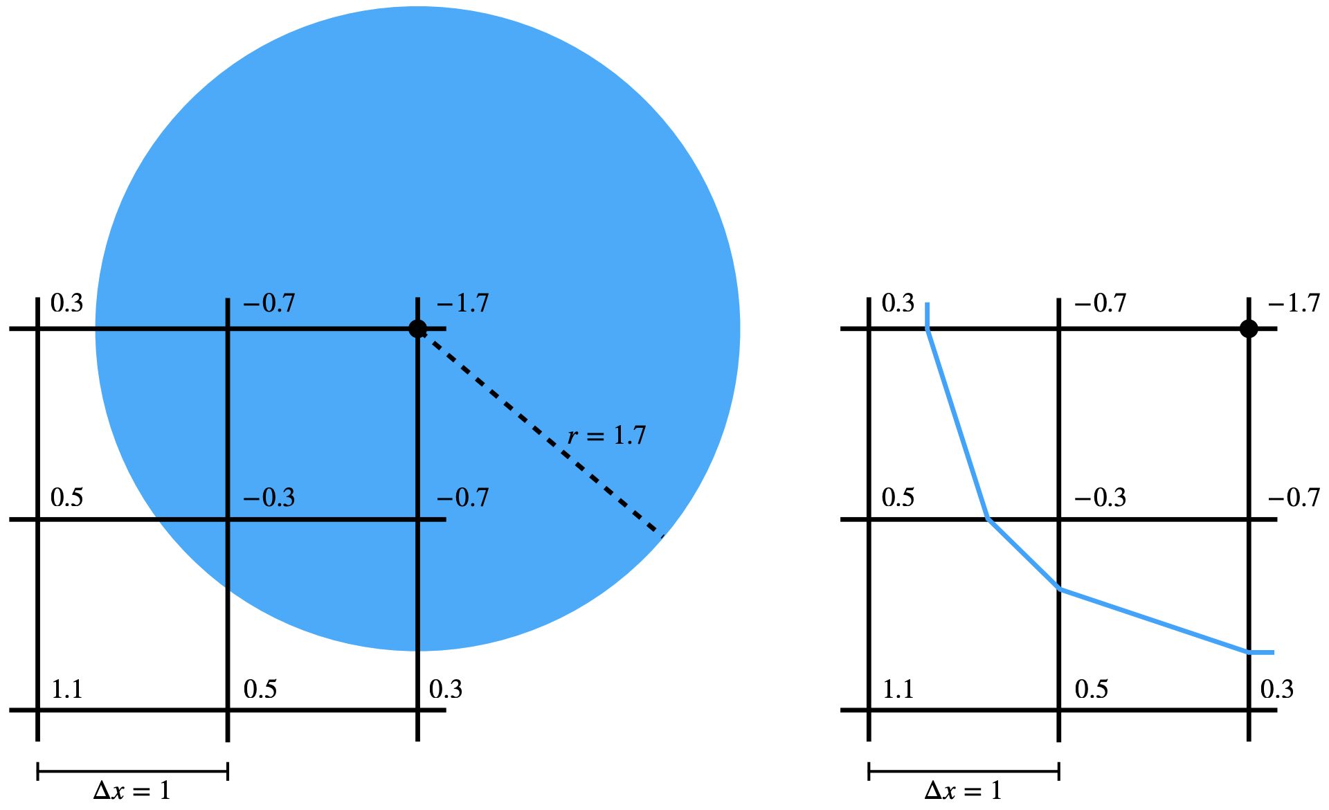
Example 7.1.3 (Grid Signed Distance Field). For a signed distance field stored on a uniform Euclidean grid with spacing \(\Delta x\), to query the distance at an arbitrary location \(\mathbf{x} = (x,y)\) where \(x = x_i + \alpha \Delta x\) and \(y = y_i + \beta \Delta x\) (\(\mathbf{x}_{i,j} = (x_i, y_j)\) are the location of grid nodes, \(0 \leq \alpha,\beta \leq 1\)), with bilinear interpolation (Figure 7.1.1 right), $$d(\mathbf{x})=(1-\beta )((1-\alpha )d({\mathbf{x}}_{i,i})+\alpha d({\mathbf{x}}_{i+1,i}))+\beta ((1-\alpha )d({\mathbf{x}}_{i,i+1})+\alpha d({\mathbf{x}}_{i+1,i+1})).$$ From Figure 7.1.1 we also see that to approximate a solid boundary smoothly in this setting, a higher-order interpolation scheme such as quadratic b-spline interpolation is needed.