Self-Contact

With triangle discretization, the boundary of the domain is approximated as a polyline formed by a set of edges. Let us denote this set of boundary edges as $E$ , and the barrier potential becomes:

$\approx = \int_{Γ_{C}} \frac{1}{2} b (X_{2} \in Γ_{C} - N (X) min ∥ x (X, t) - x (X_{2}, t) ∥, \hat{d}) d s (X) \int_{Γ_{C}} \frac{1}{2} b (e \in E - I (X) min X_{2} \in e min ∥ x (X, t) - x (X_{2}, t) ∥, \hat{d}) d s (X) \int_{Γ_{C}} \frac{1}{2} b (e \in E - I (X) min d^{PE} (x (X, t), e), \hat{d}) d s (X) .$

Here, $I (X)$ is the set of edges that contain $X$ . Completely ignoring these edges is a specific choice of $N (X)$ under the current discretization. The term $min_{X_{2} \in e} ∥ x (X, t) - x (X_{2}, t) ∥$ is simply the point-edge distance $d^{PE} (x (X, t), e)$ , which can be calculated as either a point-point distance or a point-line distance depending on the relative positions of the point and the edge.

As we know, the barrier energy density function $b$ is already a smooth approximation to the discontinuous normal contact forces that prevent interpenetration between two colliding points. However, when considering self-contact between discrete surfaces (piecewise linear here), the non-smooth $min$ operator on point-edge distances is inevitable. This non-smoothness can still pose challenges for optimization time integrators.

To obtain a smooth barrier potential even in the case of piecewise linear boundaries, we first transform the $min$ operator to a $max$ operator, as the energy density function $b$ is a non-ascending function everywhere in the domain. This gives us:

$\int_{Γ_{C}} \frac{1}{2} e \in E - I (X) max b (d^{PE} (x (X, t), e), \hat{d}) d s (X) .$

Next, we need to smoothly approximate the $max$ operator. A straightforward choice is to use the smooth max function, such as the $p$ -norm function:

$max (a_{1}, a_{2}, ..., a_{n}) \approx (a_{1}^{p} + a_{2}^{p} + \dots + a_{n}^{p})^{\frac{1}{p}},$

with $p > 0$ sufficiently large. However, the exponent $\frac{1}{p}$ will couple multiple inputs together, increasing the stencil size and making the Hessian less sparse, which will make the simulation more computationally expensive.

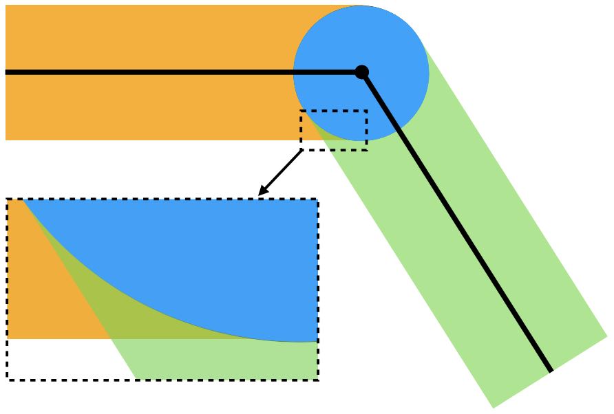
Fortunately, due to the local support of $b$ , where the contact force only exists for distances smaller than $\hat{d}$ , using $p = 1$ is sufficient. With a relatively small $\hat{d}$ , there will only be some redundant contact forces at the interface of boundary elements (Figure 20.3.1).

**Figure 20.3.1.** In this simple two-edge illustration, the yellow and green regions are only counted once by the summation, but the blue region and the yellow-green overlap are counted twice. If we subtract once the blue region, then for the right-top boundary (convex), it becomes perfect, but for the left-bottom boundary (concave), we can still see some overlap that are counted twice.

Since the overlapping supports of $b$ from multiple boundary elements can be clearly identified, it is also possible to subtract the redundant barrier potentials in those regions, as discussed in detail in [Li et al. 2023]. For this book, let us keep it simple by using $p = 1$ with the $p$ -norm formulation, which is just summation:

$\int_{Γ_{C}} \frac{1}{2} e \in E - I (X) max b (d^{PE} (x (X, t), e), \hat{d}) d s (X) \approx \int_{Γ_{C}} \frac{1}{2} e \in E - I (X) \sum b (d^{PE} (x (X, t), e), \hat{d}) d s (X) .$

Approximating the integral under triangle discretization and picking the end points of each boundary edge as the quadrature points, we obtain the fully discrete form:

$\approx \int_{Γ_{C}} \frac{1}{2} e \in E - I (X) \sum b (d^{PE} (x (X, t), e), \hat{d}) d s (X) \overset{a}{^} \sum \frac{∥ X _{\overset{a}{^}} - X _{\overset{a}{^} - 1} ∥ + ∥ X _{\overset{a}{^}} - X _{\overset{a}{^} + 1} ∥}{4} e \in E - I (X_{\overset{a}{^}}) \sum b (d^{PE} (x_{\overset{a}{^}}, e), \hat{d}) . (20.3.1)$

Similar to the solid-obstacle contact cases, $T_{C}$ can be derived by taking the derivative of the whole contact potential with respect to the nodal degrees of freedom (DOFs).