Distance Barrier

Constrained Optimization

In scenarios like a solid interacting with a planar ground, where the signed distance function $ d(\mathbf{x}) $ is smooth outside the obstacle, we can approach the modeling of contact by incorporating non-interpenetration constraints. These constraints are formulated using $ d(\mathbf{x}) $, while we also aim to minimize the Incremental Potential of the system.

Assuming that the solids are densely sampled with nodes $\mathbf{x}$, we apply these constraints at the level of nodal Degrees of Freedom (DOFs) in relation to the obstacles:

$x min E (x) s.t. d_{ij} \geq 0 \forall node i and obstacle j . (7.2.1)$

In this equation, $ d_{ij} $ represents the signed distance between node $ i $ and obstacle $ j $. By ensuring that $ d_{ij} $ is non-negative, we effectively prevent the solids from intersecting with the obstacles¹.

Logarithm Barrier Potential in Contact Modeling

To address the inequality constraints in our contact modeling, we introduce a barrier potential $ P_b(\mathbf{x}) $. This potential transforms the constrained problem, as described in Equation (7.2.1), into an "unconstrained" optimization problem:

$x min E (x) + h^{2} P_{b} (x) . (7.2.2)$

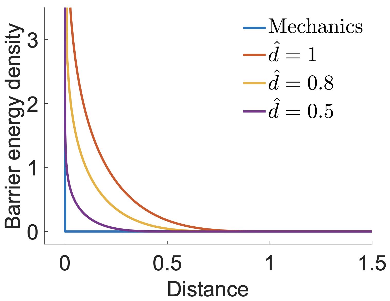
The barrier potential is defined as follows:

$P_{b} (x) = i, j \sum A_{i} \hat{d} b (d_{ij} (x)) and b (d_{ij} (x)) = {\frac{κ}{2} (\frac{d _{ij}}{d ^} - 1) ln \frac{d _{ij}}{d ^} 0 d_{ij} < \hat{d} d_{ij} \geq \hat{d} . (7.2.3)$

In this formulation, $ b() $ represents the barrier energy density function. As the distance approaches zero, this function tends to infinity, thereby providing a strong repulsion force to prevent interpenetration (refer to Figure 7.2.1). The distance threshold $ \hat{d} $ above which no contact force is exerted, the contact stiffness $ \kappa $ which controls the rate of change of the contact forces with respect to distance, and $ A_i $, the contact area of node $ i $, are key parameters in this setup. By integrating the energy density over the solid boundary, the barrier formulation effectively models a potential energy field that is of thickness $ \hat{d} $.

**Figure 7.2.1.** The barrier energy density function plotted with different $\hat{d}$ . Decreasing $\hat{d}$ asymptotically matches the discontinuous definition of the contact condition.

Remark 7.2.1 (Contact Layer Interpretation). Imagine the barrier potential $ P_b(\mathbf{x}) $ as representing the elasticity of an ultra-thin layer of virtual material that exists just outside the boundaries of the solids. This virtual layer has an effective thickness of $ \hat{d} $, which correlates with the distance threshold in the barrier function.

Consequently, the integration or summation used in computing $ P_b(\mathbf{x}) $ is weighted by the volume element $ w_i = A_i \hat{d} $, where $ A_i $ represents the contact area of each node. As solids approach and begin to compress this virtual elastic layer, contact forces arise. These forces, akin to a unique type of elasticity force, serve to prevent interpenetration by providing a repulsion effect whenever the solids come too close to each other. This model allows us to simulate the physical response of contact without actual penetration of the solids.

Applying chain rules with distance being the intermediate variables, we can derive the gradient and Hessian of $P_b(\mathbf{x})$ as $\nabla P_{b} (x) = i, j \sum w_{i} \frac{\partial b}{\partial d} (d_{ij} (x)) \nabla d_{ij} (x) (7.2.4)$ and $\nabla^{2} P_{b} (x) = i, j \sum w_{i} (\frac{\partial ^{2} b}{\partial d ^{2}} (d_{ij} (x)) \nabla d_{ij} (x) \nabla d_{ij} (x)^{T} + \frac{\partial b}{\partial d} (d_{ij} (x)) \nabla^{2} d_{ij} (x)) . (7.2.5)$

As we are using signed distances here, the inequality constraints can be defined without introducing an $\epsilon$ as in Equation (2.3.1) with unsigned distances.